Using Note Assist QA you can run clinical documentation downloaded from your system against a Note Assist review to identify gaps in required information. This powerful feature helps you quickly spot documentation issues and determine which clinicians may benefit from targeted coaching.
Information from Note Assist QA is not saved in nVoq Administrator, and does not count towards Note Assist usage.
Run Note Assist QA
Label-based categories are not currently supported with Note Assist QA.
If your review includes label-based categories when you run Note Assist QA, the system will display an error indicating it can’t run the review. To proceed, remove any label-based categories before running Note Assist QA. This will be fixed in an upcoming release of nVoq Administrator.
- Run a batch file of narratives from your EMR against a Note Assist review to see if existing narratives match review categories.Information from these review is not saved in nVoq Administrator and does not count towards Note Assist usage.
- Do a bulk export of patient narratives from your EHR -OR- create your own review file using our template.
- Prepare exported data for the review:
- Pull out any narratives you do not want to include in the review.
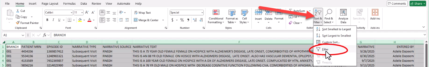
- In Microsoft Excel, select the entire spreadsheet by clicking on the Select All button. That's the arrow in the top left corner of the spreadsheet (between the first column and the first row).

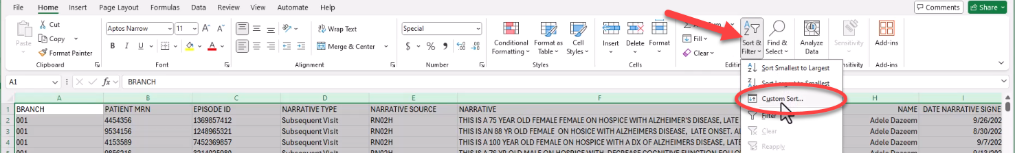
- Add filters to each column header. Click the Sort & Filter button on the toolbar, then select the Filter option.
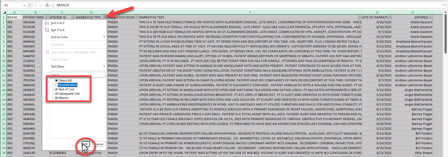
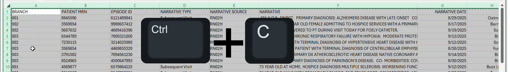
- On the column that displays the narrative type, click the drop-down arrow next to the header to open the filter, and uncheck the box next to any of the listed narrative types you do not want to include in the review. Then click the OK button.
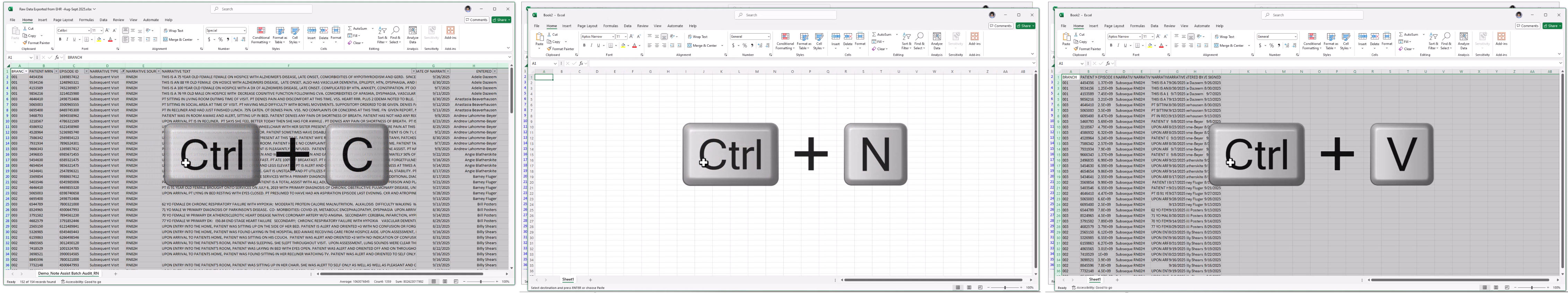
- With only the narrative types you want in the file and the entire spreadsheet still selected, click Crtl+C on your keyboard (to copy selected narratives), and Ctrl+N (to create a new spreadsheet), and then Ctrl+V (to paste copied data into the new spreadsheet). This new spreadsheet is the one you will run in Note Assist QA.
- Name your new file and save it in a HIPAA-compliant location. This may be the hard drive on your computer. Do not save it to a shared network folder.
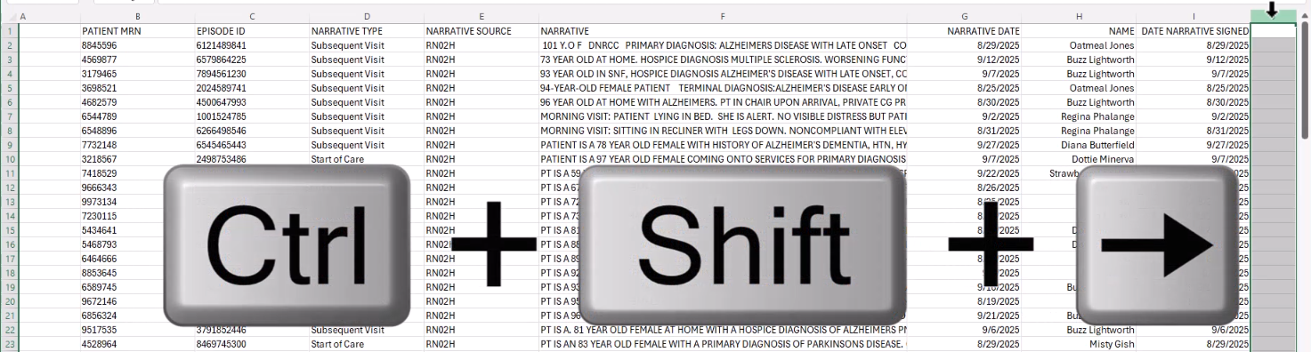
- In Microsoft Excel, select the entire spreadsheet by clicking on the Select All button. That's the arrow in the top left corner of the spreadsheet (between the first column and the first row).
- Ensure that your file has the three required headers/columns:
- Your file must include - in any order - three column headers: Narrative Date, Narrative, and Name.

- The Narrative Date column includes the date that the narrative was created. The header name is not case-sensitive. Other header names, such as "Narrative Signed Date" may also be accepted. The information in this column needs to be a date, but many formats of date (including dates with time and milliseconds) are accepted.
- The Narrative column includes the actual patient narrative text. The header name is not case-sensitive. Other header names, such as "Narrative Text" may also be accepted.
- The Name column includes the name of the clinician who created the narrative. The header name is not case-sensitive. Other header names, such as "Worker" may also be accepted. The clinician named here does not need to have a corresponding nVoq account.
- Your file can have any additional columns that might be helpful for you when analyzing the data. These will be ignored by the system, but will still appear in the output file.

- All columns must have a header.
- Combined column headers (merged cells) should be split out so that every column has its own header.
- Save your file.
- Your file must include - in any order - three column headers: Narrative Date, Narrative, and Name.
- Eliminate any hidden formulas that may be in your file from the extraction process from your EHR to prevent errors during processing.
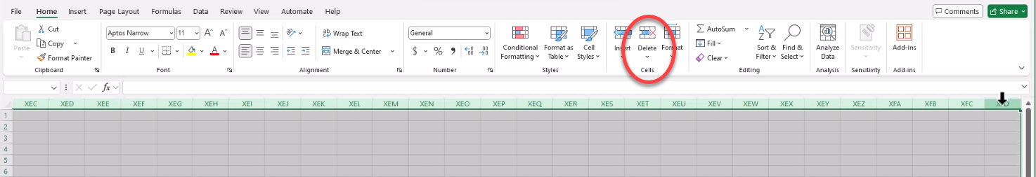
- Select the first column that has no data.
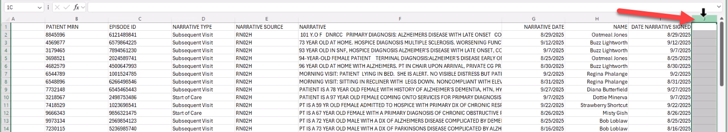
- With the column selected, press Ctrl+Shift+Right key on your keyboard.
- Click Delete on the Excel toolbar to delete all of the columns that may have hidden data.
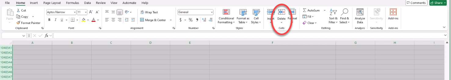
- Select the first row that has no data.

- With the row selected, press Ctrl+Shift+Down key on your keyboard.
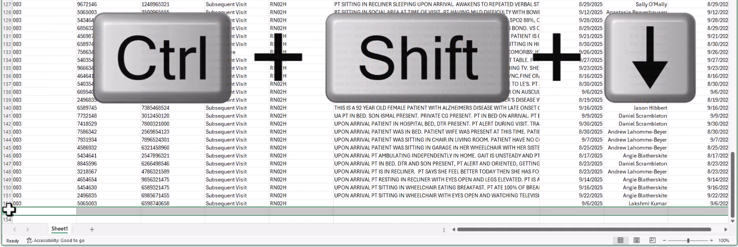
- Click Delete on the Excel toolbar to delete all of the rows that may have hidden data.
- Save your file.
- Select the first column that has no data.
- Make sure all narrative cells have data in them. (You may have some that are empty.)
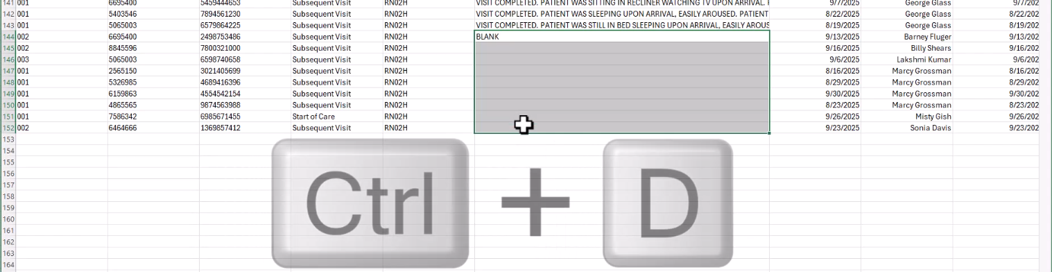
- Type the word "BLANK" in each empty narrative cell to show that noting was recorded by the clinician and to ensure you do not receive the "missing value" error from nVoq Administrator.
To quickly do this:- Click the Sort & Filter button in the Excel toolbar, then select Custom Sort.
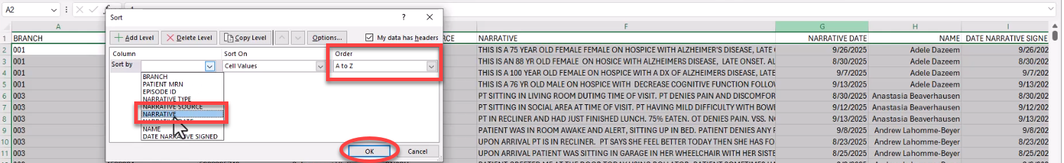
- In the Sort window that opens, select Narrative from the Column menu, and make sure the Order menu has A to Z selected. Then click OK.
- Scroll down to the empty narrative cells. Type "BLANK" in the first empty narrative cell, then select that cell and the rest of the empty narrative cells, and use Ctrl+D to fill down.
- Click the Sort & Filter button in the Excel toolbar, then select Custom Sort.
- Save your file.
- Type the word "BLANK" in each empty narrative cell to show that noting was recorded by the clinician and to ensure you do not receive the "missing value" error from nVoq Administrator.
- Pull out any narratives you do not want to include in the review.
- Run the review in nVoq Administrator:
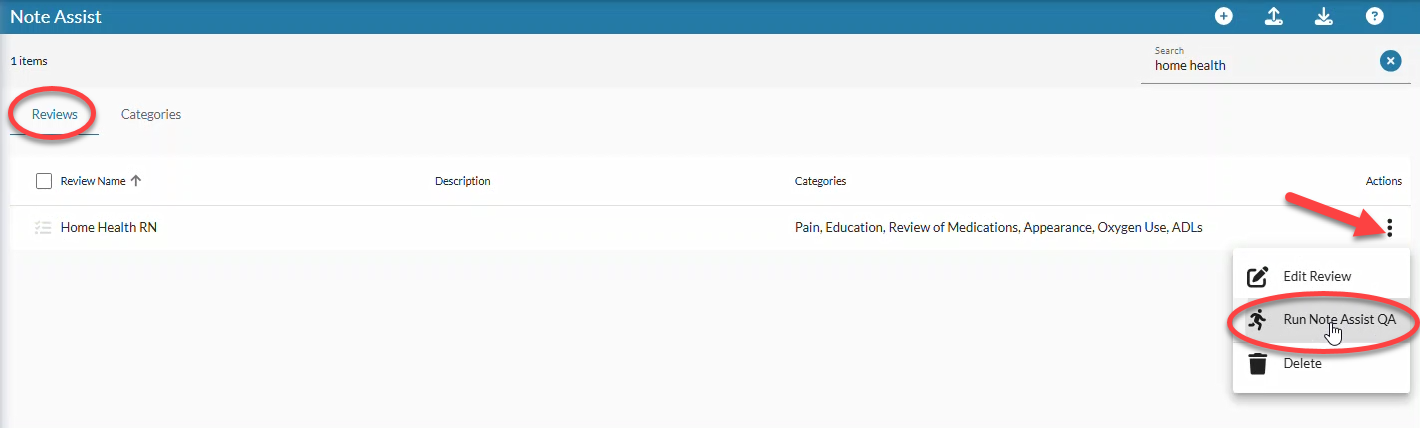
- On the Note Assist page Reviews tab, click the actions menu next to the review you want to run a batch file against and select Run Note Assist QA.
 OR double-click on the review to open the Edit Note Assist Review page, then click the Run Note Asssit QA icon
 in the blue toolbar.
- On the Run Note Assist QA page, click on the Choose a file link in the dotted line box and navigate to your saved file, OR drag your file from an open directory into the dotted line box.
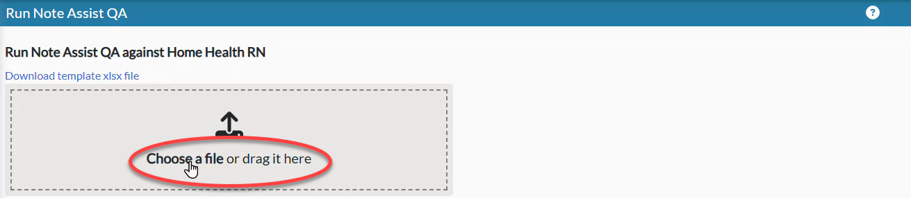
- The maximum file size is 6MB.
- Run the review against one file at a time.
- Only the first sheet in the file will be included in the review run; any additional sheets will be ignored.
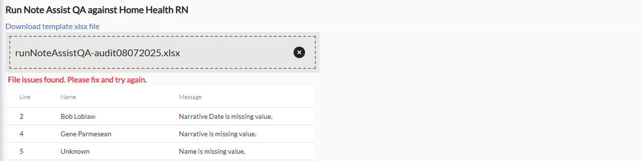
- The system will check the file for missing required columns, column names, or data, and to make sure it does not exceed the maximum file size.
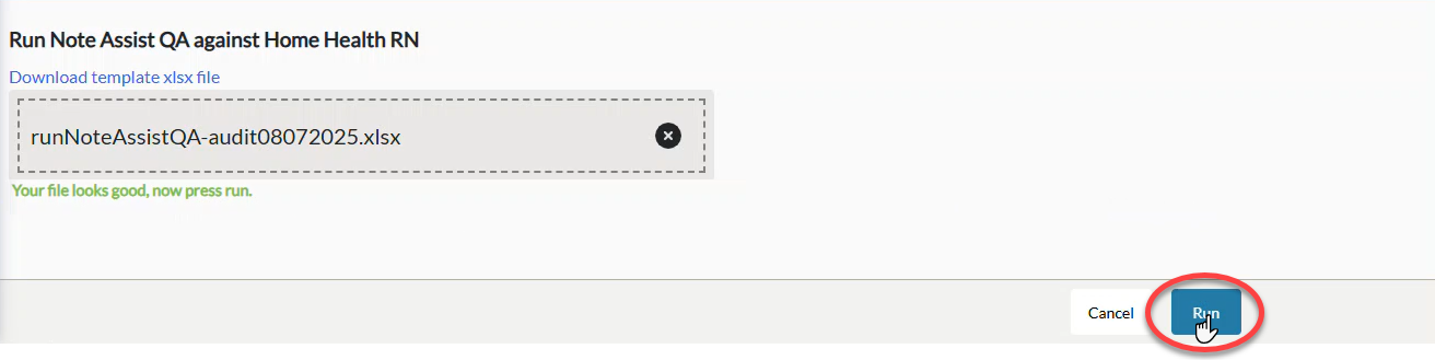
- If no issues exist, go to step 3d.
- If information is missing or the file is too large that information will be presented below the file box. Click the X next to the file name to remove it from the page, fix the errors in the file, and then try the upload again.
- When your file looks good, click the Run button.
- On the Note Assist page Reviews tab, click the actions menu next to the review you want to run a batch file against and select Run Note Assist QA.
- When processing is complete your output file is downloaded automatically to your local Downloads folder.
- The output file name is the same as the original file name prepended with the current date.
- If the file was unable to run you will see a red popup notification explaining why the batch request was unable to run, and that information is also available in the notifications list.

- Do a bulk export of patient narratives from your EHR -OR- create your own review file using our template.
Analyze Review Results
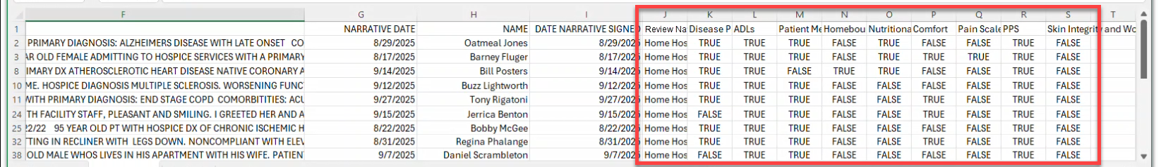
- Go to your Downloads folder to open the output file. The output file includes:
- The Narrative, Narrative Date, and Name columns
- Any extra columns that were included in the original file
- A column for the Audit Name, which is the review that the batch was run against
- A column for each category in the review. Each category cell shows either TRUE (if the category was included in the Narrative text) or FALSE (if the category was missing from the Narrative text) for each narrative in the report.
- Click the Enable Edit button near the top of the Excel file.

- Rename the sheet that includes the results to Review Results.

- Double-click on the text on the tab.
- Type over the original tab name.
- Click on the New Sheet icon near the sheet tab to create a second sheet.

- Name the new sheet Analysis.

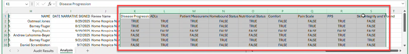
- Copy the data from the Review Results sheet to the Analysis sheet. This gives you a place to analyze the data without changing the formatting of the original results.
- Select the entire Review Results sheet by clicking on the Select All button in the top left corner of the spreadsheet (between the first column and first row).

- Press Ctrl+C on your keyboard to copy the selected data.
- Click the Analysis tab.

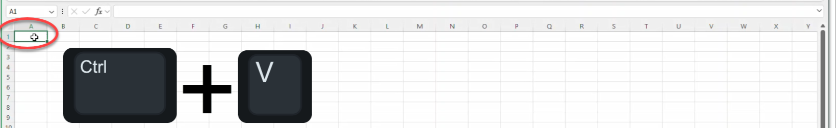
- Place your cursor in cell A1 and then press Ctrl+V to paste the review results into the Analysis sheet.
- Select the entire Review Results sheet by clicking on the Select All button in the top left corner of the spreadsheet (between the first column and first row).
- Make the category data numerical.
- Select all of the category columns.
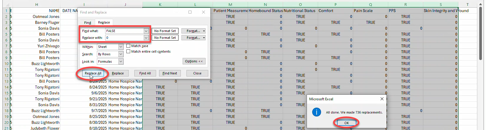
- Press Ctrl+H on your keyboard to open the Find and Replace window.
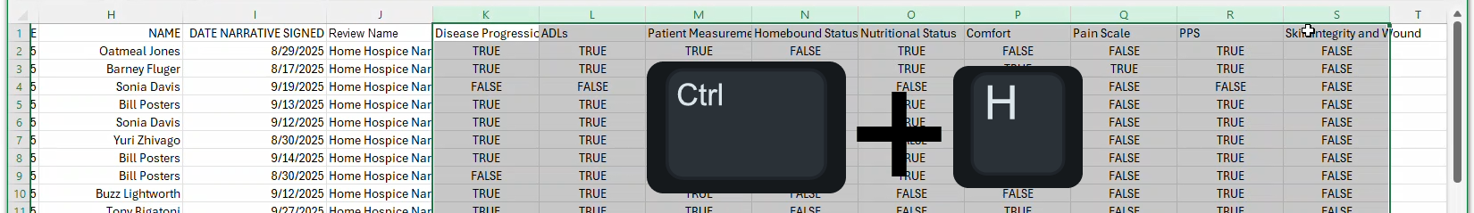
- In the Find and Replace window on the Replace tab, type FALSE in the Find What box, and 0 (zero) in the Replace With box. Then click the Replace All button. Click OK to close the message that tells you how many replacements were made.
- Still in the Find and Replace window on the Replace tab, type TRUE in the Find What box, and type 1 (one) in the Replace With box. Then click the Replace All button. Click OK to close the message that tells you how many replacements were made.
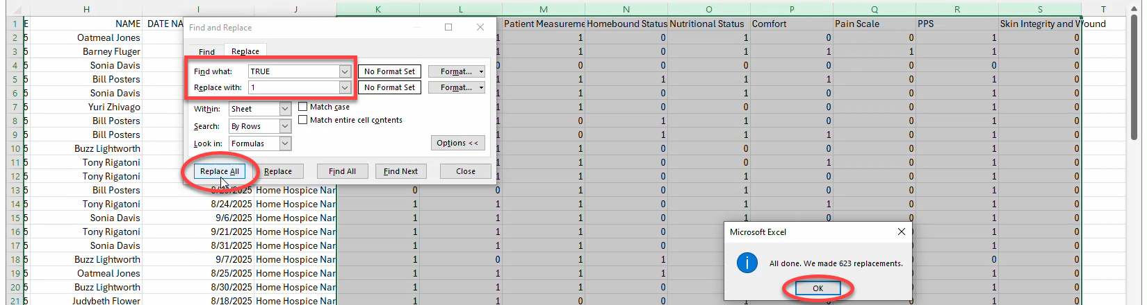
- Close the Find and Replace window.
- Select all of the category columns.
- Add highlighting to category data cells to make it easier to differentiate the results.
- Select all of the category columns. (They may still be selected from the previous step.)
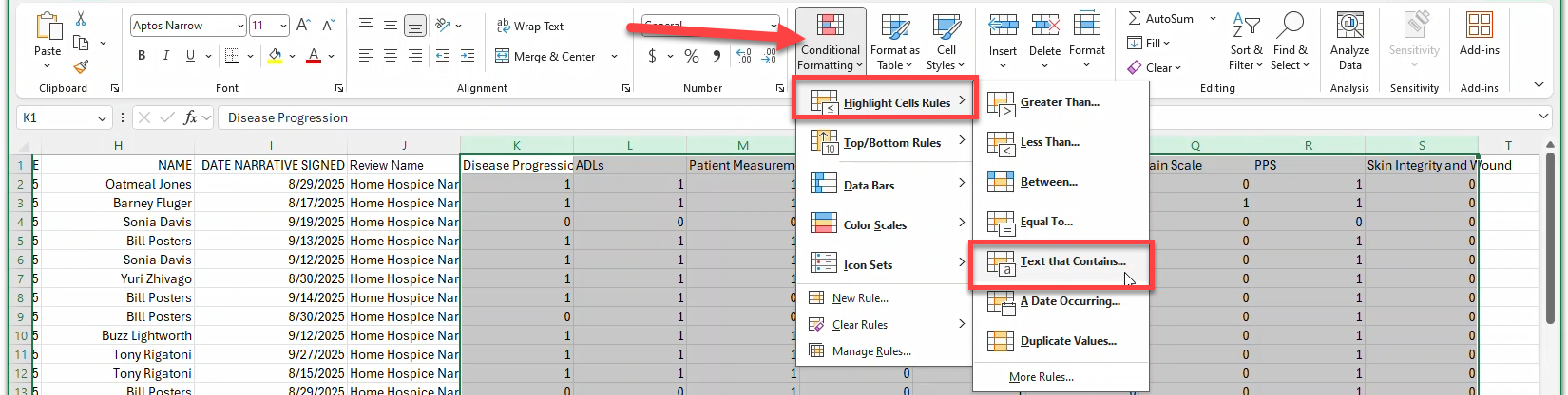
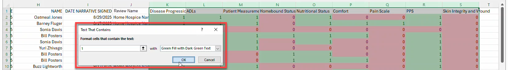
- In the Excel toolbar Styles section, click Conditional Formatting, select Highlight Cell Rules, and then select Text that Contains.
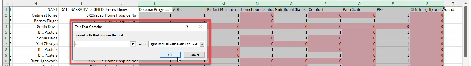
- In the Text That Contains window, type 0 (zero) in the Format cells that contain the text box, and select Light Red Fill with Dark Red Text on the with menu (this may already be selected by default). Click the OK button.
- With category columns still selected, again click Conditional Formatting and select Highlight Cell Rules, and then select Text that Contains.
- This time type 1 (one) in the Format cells that contain the text box, and select Green Fill with Dark Green Text on the with menu. Click the OK button.
- Calculate the total "score" for each narrative.
- In the first blank column header to the right, type Total.

- Select all of the numerical column results for the first narrative (in Row 2).

- Click the AutoSum button (in the Editing section of the toolbar).
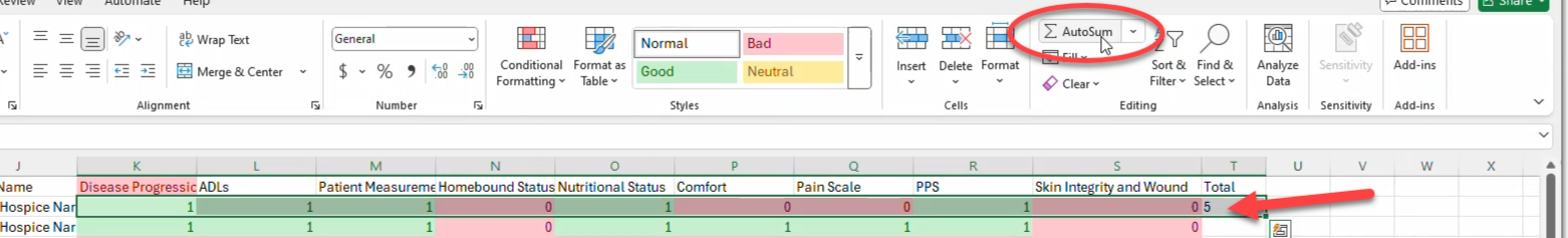
- Double-click the lower right corner of the cell showing the sum. This will carry the AutoSum function down through the remaining rows.
- In the first blank column header to the right, type Total.
- Put a filter on all of the data in the sheet so you can filter on anything as you analyze results.
- Select all columns with data.
- Click Sort & Filter (in the Editing section of the toolbar), and select Filter.
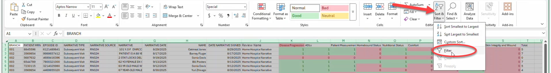
- This adds the filter drop-down to all selected columns.

- Calculate the sums and percentages of each category that was met in the review.
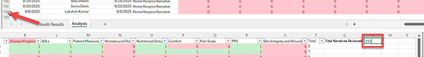
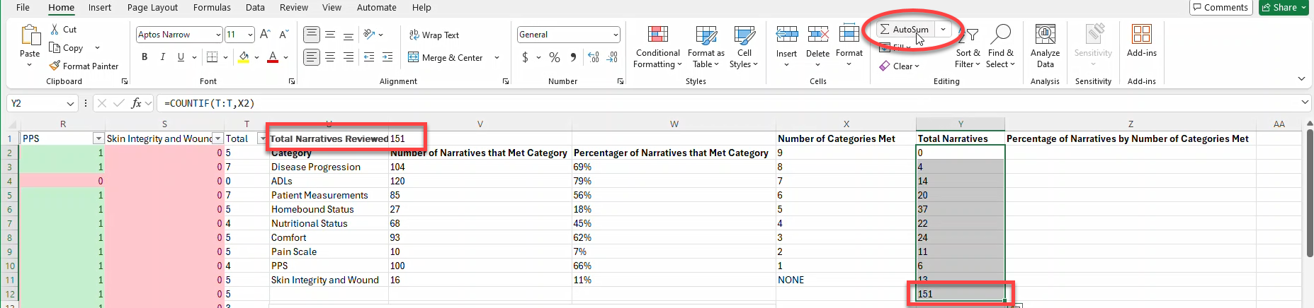
- In one cell type Total Narratives Reviewed.
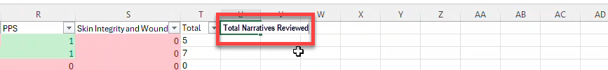
- In the cell next to that, enter the total number of narratives that were reviewed. (The total number of narratives reviewed is one less than the total number of rows of data on your spreadsheet.)
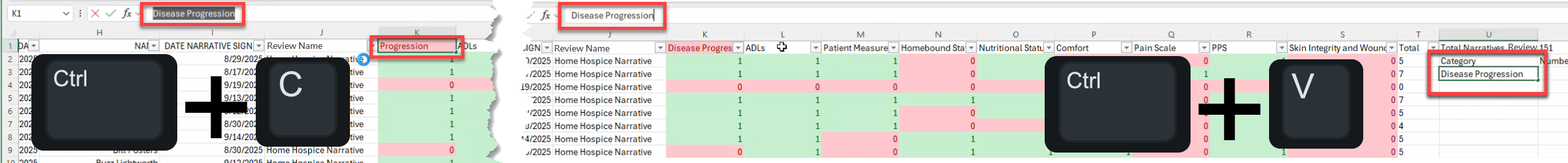
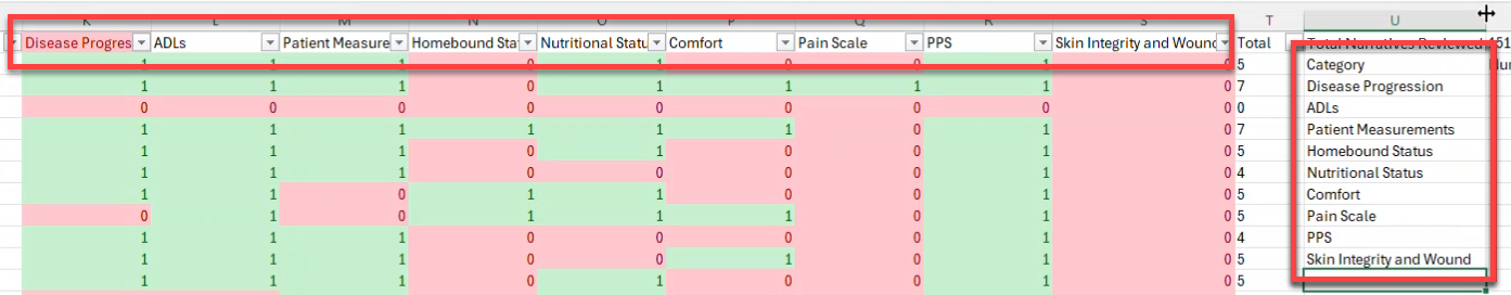
- Below your Total Narratives Reviewed, add three columns titles: Category, Number of Narratives that Met Category, and Percentage of Narratives that Met Category.

- Below the Category column, copy and paste the name of each category in a separate cell.
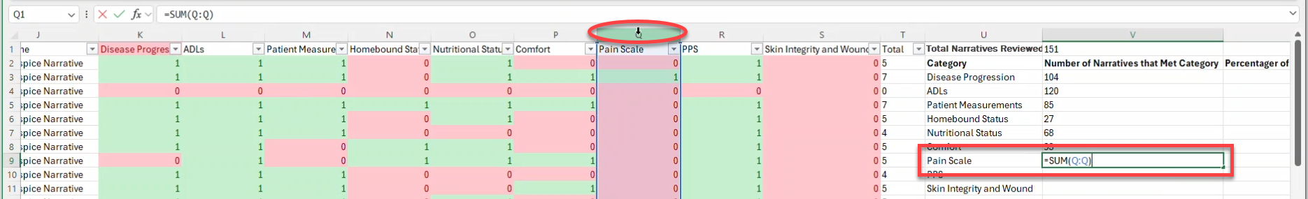
- Place your cursor in the first cell below the Number of Narratives that Met Category column heading and enter =SUM( then click on the letter at the top of the corresponding category column. Finally add ) (closing parenthesis) to your formula, then press Enter on your keyboard. You'll end up with something like this: =SUM(F:F)
- Repeat for each category below the Number of Narratives that Met Category heading.
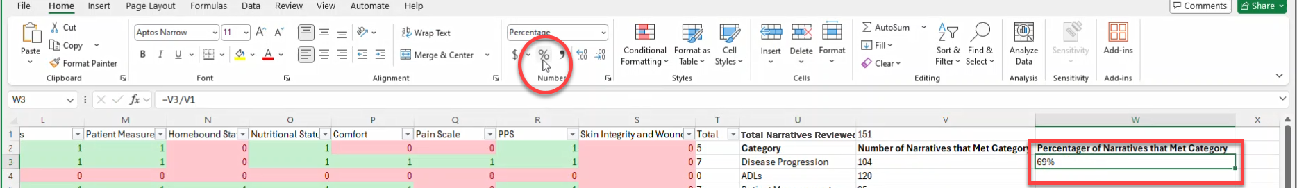
- Place your cursor in the first cell below the Percentage of Narratives that Met Category column heading and enter = (equal sign) then click on the cell that includes the Number of Narratives that Met Category for that row. Enter / (forward slash) and then click on the number of Total Narratives Reviewed and press Enter on your keyboard. So you will have something like this: =Q3/Q1

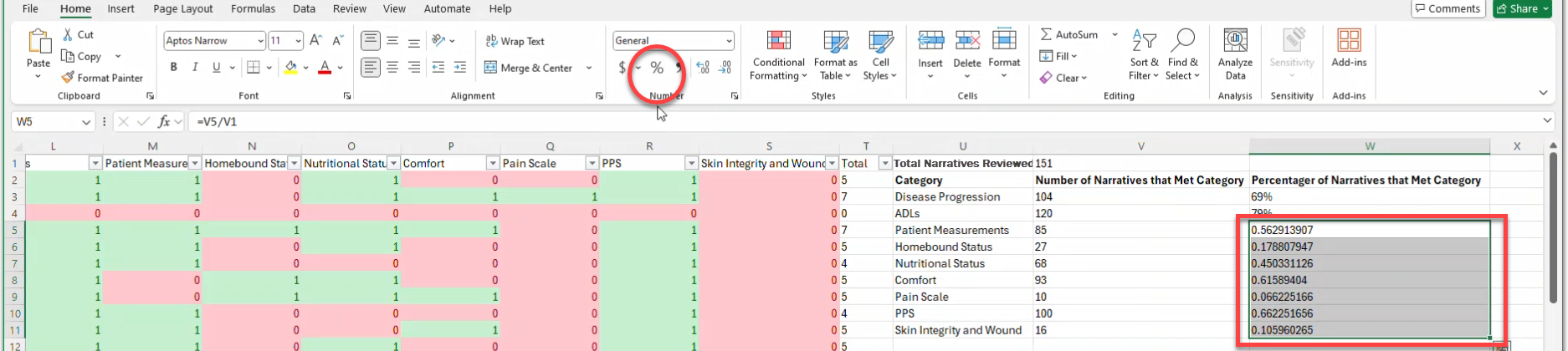
- With your cursor on the cell of the formula you just entered, click the % button (in the Number section of the Excel toolbar) to change the result in that cell from a decimal to a percentage.
- Repeat the previous two steps for each category below the Percentage of Narratives that Met Category heading.
- In one cell type Total Narratives Reviewed.
- Create a chart of the data from the sums and percentages of each category met.
- Select the cells that include the data you just created (below the Total Narratives Reviewed) and click the Quick Analysis icon that appears in the lower right corner of the selected cells.
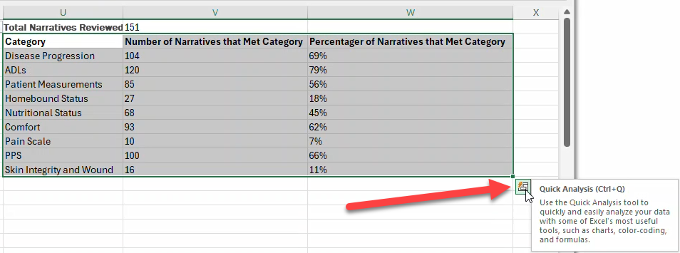
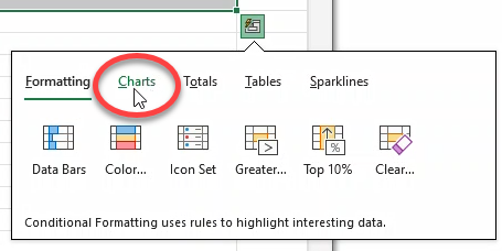
- On the menu that opens, select Charts.
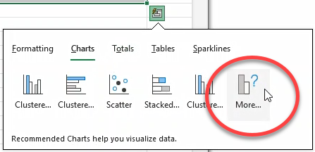
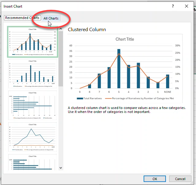
- Click More to open the Insert Chart window and see all of the charts you have available.
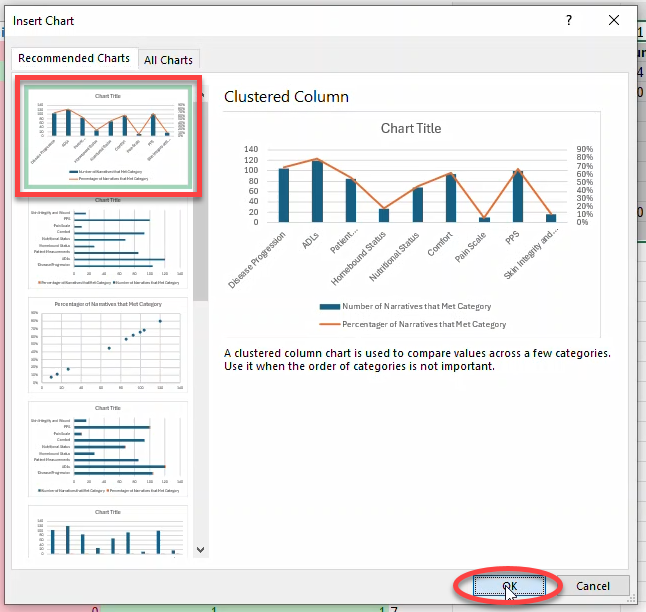
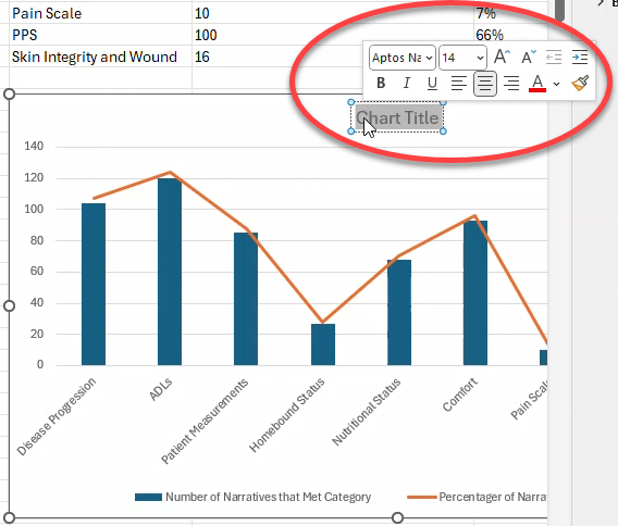
- In the Insert Chart window, select the chart you want to create (in this example I have selected Clustered Column), then click OK.
- Drag the chart anywhere you want it on the sheet, and resize by dragging the chart area handles.
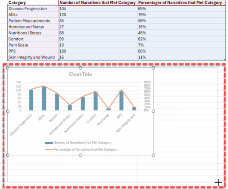
- Double-click the Chart Title text and type over it to add an appropriate chart title.
- Select the cells that include the data you just created (below the Total Narratives Reviewed) and click the Quick Analysis icon that appears in the lower right corner of the selected cells.
- Calculate the number of categories met, number of total narratives, and percentage of narratives by number of categories met.
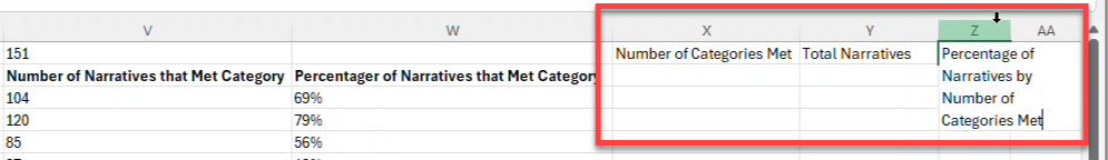
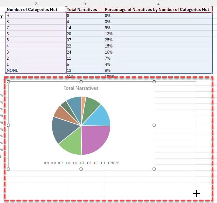
- Add three columns with the following headers: Number of Categories Met, Total Narratives, and Percentage of Narratives by Number of Categories Met.
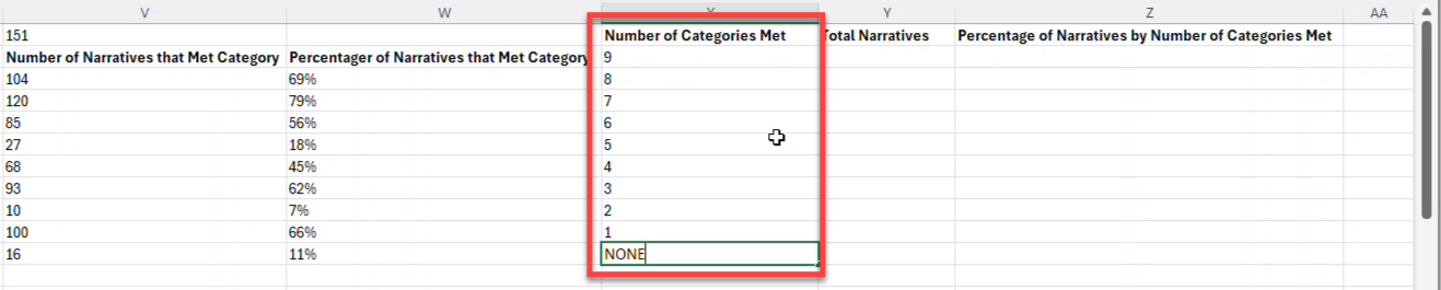
- Under the Number of Categories Met column enter the total number of categories in this review in the first cell, then count down to 1 in each cell under that. For the final cell (below 1) type NONE.
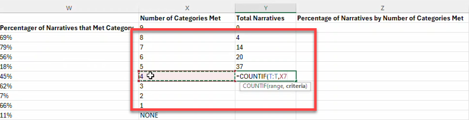
- Select the first cell below Total Narratives and enter =COUNTIF( then click on the letter of the Total column, add a comma (,) and then click on the cell that includes the first Number of Categories Met. Finally add ) (closing parenthesis) and press Enter, so you end up with something like =COUNTIF(N:N,P14)

- Repeat that process for each cell below to ensure the formula incorporates the cell to the left.
 When you get to the final cell (next to NONE) instead of selecting the cell, type 0 (zero) in the formula. (For example, =COUNTIF(N:N,0)
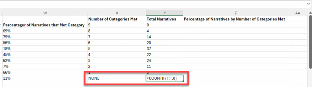
- To make sure the math is correct, sum up the Total Narratives column and make sure you get the same as the Total Narratives Reviewed: select all of the totals in the column you just created and then click the AutoSum button. It should be the same as the Total Narratives Reviewed.
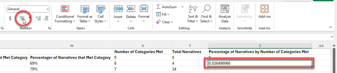
- Place your cursor in the first cell below the Percentage of Narratives by Number of Categories Met column heading and enter = (equal sign). Click on the cell that includes the Total Narratives number for that row, enter / (forward slash) and then click on the cell that includes the Total Narratives Reviewed number and press Enter on your keyboard. For example, =Q3/Q1

- With your cursor on the cell of the formula you just entered, click the % button (in the Excel toolbar) to change the result in that cell from a decimal to a percentage.
- Repeat the previous step for each of the number of categories met rows below the Percentage of Narratives by Number of Categories Met heading. (Copying and pasting the formula does not work here.)
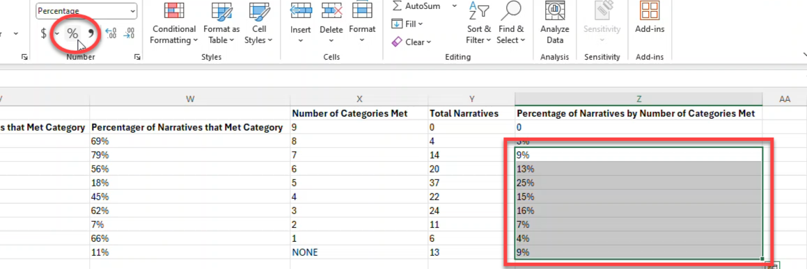
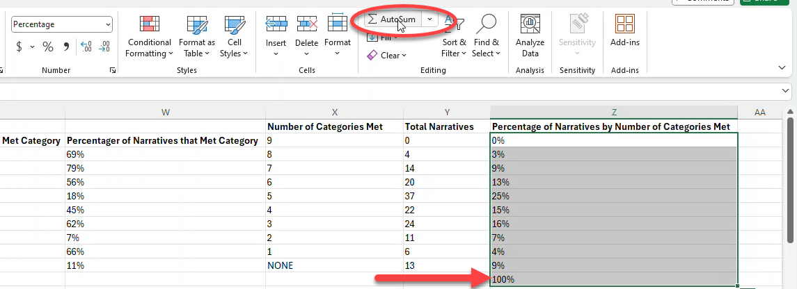
- To make sure your math is correct use AutoSum again to sum the percentages you just added and make sure you get 100%.
- Add three columns with the following headers: Number of Categories Met, Total Narratives, and Percentage of Narratives by Number of Categories Met.
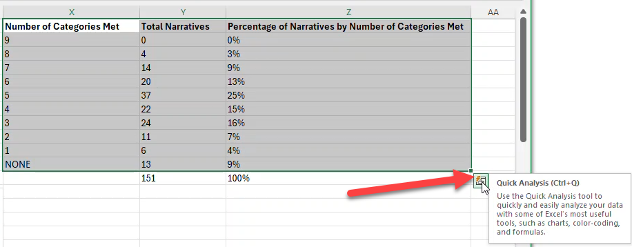
- Create a chart of the data from number of categories met, number of total narratives, and percentage of narratives by number of categories met.
- Select the cells that include the data you just created (do not include the sums at the bottom) and click the Quick Analysis icon that appears in the lower right corner of the selected cells.
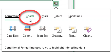
- On the menu that opens, select Charts.
- Click More to open the Insert Chart window.
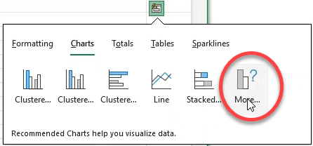
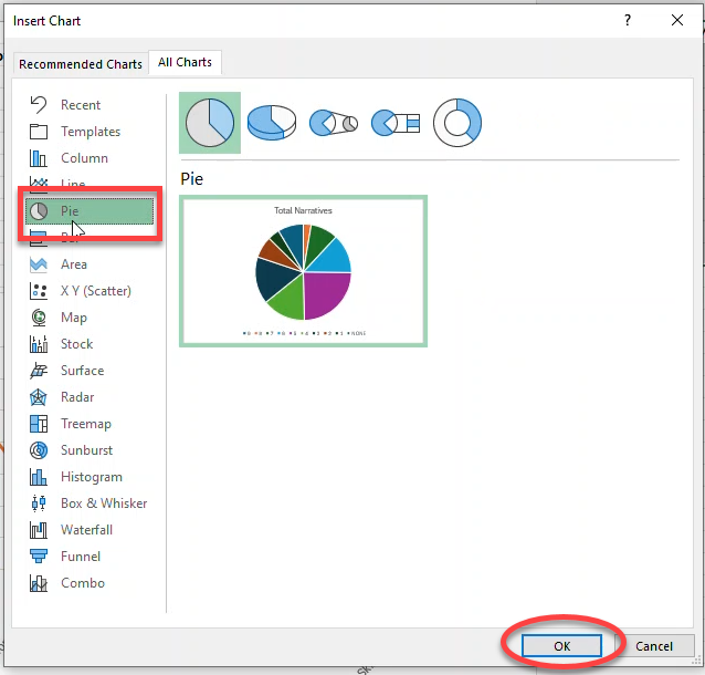
- On the Insert Chart window, click the All Charts tab.
- Select Pie, then click the OK button.
- Drag the chart anywhere you want it on the sheet, and resize by dragging the chart area handles.
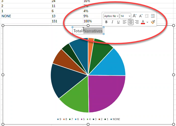
- Add an appropriate chart title by double clicking on the Chart Title text, selecting it, and typing over it.
- Select the cells that include the data you just created (do not include the sums at the bottom) and click the Quick Analysis icon that appears in the lower right corner of the selected cells.
Download the Note Assist QA Review Template
On the Run Note Assist QA page, use the Download template xlsx file link to create your own file.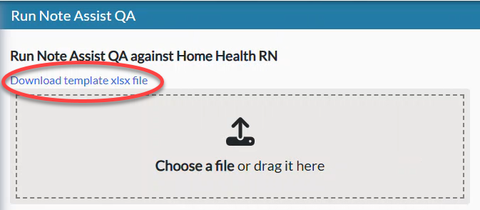
- The template includes the columns required for Note Assist QA:
- Narrative - The clinical note text that will be run against the selected review.
- Narrative Date - The date that the narrative was created.
- Name - The name of the person who created the narrative. This name does not need to have a corresponding nVoq account.